2. Approaches to Valuation
Approaches to Valuation
1. Discounted Cashflow Valuation
- The the value of an asset to the present value of expected future cashflows on that asset
- the value of any aset is the present value of expected future cashflows that the asset generates
\( value\ =\ Σ^{t=n}_{t=1}\frac{CF_t}{(1+r)^t}\) r : reflecting the riskiness of estimated cashflows
Categorizing DCF Models
- equity valuation - value just the equity stake in the business (residual cashflows after metting all expenses, reinvestment needs , tax obligations and net debt payments
\[value\ of\ equity = Σ^{t=n}_{t=1}\frac{CF\ to\ equity_t}{(1+k_e)^t}, k_e:\ cost\ of \ equity\]
- Firm valuation - value the entire firm, (residual cashflows after metting all operating expenses, reinvestment needs and taxes, but prior to any payments to either debt or equity holders
\[value\ of\ firm = Σ^{t=n}_{t=1}\frac{CF\ to\ Firm_t}{(1+WACC)^t} \]
- WACC : the cost of the different components of financing used by the firm, weighted by their market value proportions
Adjusted Present Value(APV) Valuation - valuing each claim on the firm separately
- value equity -> the value added by debt by considering the PV of the tax benefit
- cost of debt = pre-tax rate (1-tax rate)
- WACC = Cost of Equity(E/(E+D)) + Cost of Debt (D/(D+E))
Applicability & Limitation of DCF Valuation
- easiest for assets whose cashflows are currently positive and can be estimated with some reliability ofr future period, and where proxy for risk that can be used to obtain discount rate is avaliable
Firms in trouble : negative earnings and cashflows & expects to lose money for some time in the future => does not work very well
Cyclical Firms : expected future cashflows are usually smoothed out, unless the analyst wants to undertake the onerous task of predicting the timing and duration of econimic recessions and recoveries
Firms with unutilized assets : If a firm has assets that are unutilized, the value of these assets will not be reflected in the value obtained from discounting expected future cashflows
Firms with patents or product option : the value will understate the true value of the firm
Firms in the process of restructuring : often change their structure, using historic data for such firm can give a misleading picture of the firm's value
Firms involved in acquisitions
private firms : no historical prices to check risk
2. Relative Valuation
- we assume that the market is correct in the way it prices stocks, on average, but that it makes errors on the pricing of individual stocks
Categorizing Relative Valuation Models
- Fundamentals versus Comparables
- Using Fundamentals - relates multiples to fundamentals about the firm being valued growth rates in earnings and cashflows, payout ratios and risk.
- Using Comparables - compare how a firm is valued with how similar firms are priced by the market
- we have to either explicitly or implicitly control for differences across firms on growth, risk and cash flow measures. In practice, controlling for these variables can range from the naive (using industry averages) to the sophisticated (multivariate regression models where the relevant variables are identified and we control for differences.)
- Cross Sectional versus Time Series Comparisons
- Cross Sectional Comparisons
- The conclusions can vary depending upon our assumptions about the firm being valued and the comparable firms
- you cannot compare firms without making assumptions about their fundamentals.
- Comparisons across time
- have to assume that your firm has not changed its fundamentals over time.
- Comparing multiples across time can also be complicated by changes in the interest rates over time and the behavior of the overall market
- Cross Sectional Comparisons
Applicability of multiples & limitations
- Given that no two firms are exactly similar in terms of risk and growth, the definition of 'comparable' firms is a subjective one. Consequently, a biased analyst can choose a group of comparable firms to confirm his or her biases about a firm's value.
- it builds in errors (over valuation or under valuation) that the market might be making in valuing these firms
3. Contingent Claim Valuation
- the value of an asset may not be greater than the present value of expected cash flows if the cashflows are contingent on the occurrence or non-occurrence of an event.
Basis for Approach
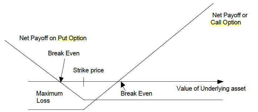
Option variables : the current value, the variance in value of the underlying asset, the strike price, the time to expiration of the option and the riskless interest rate.
The fundamental premise behind the use of option pricing models is that discounted cash flow models tend to understate the value of assets that provide payoffs that are contingent on the occurrence of an event
- if there exists undeveloped oil reserve..
- The oil company will develop this reserve if oil prices go up and will not if oil prices decline.
- The oil company will develop this reserve if development costs go down because of technological improvement and will not if development costs remain high.
When we use option pricing models to value assets such as patents and undeveloped natural resource reserves, we are assuming that markets are sophisticated enough to recognize such options and to incorporate them into the market price
Applicability of Option Pricing Models & Limitation
- Equity : call option on the value of the underlying firm, with the face value of debt representing the strike price and term of the debt measuring the life of the option
- Patent : call option on a product, with the investment outlay needed to get the project going representing the strike price and the patent life being the time to expiration of the option.
- When the underlying asset is not traded, the inputs for the value of the underlying asset and the variance in that value cannot be extracted from financial markets and have to be estimated. Thus the final values obtained from these applications of option pricing models have much more estimation error associated with them than the values obtained in their more standard applications (to value short term traded options)