4. The Basics of Risk
The Basics of Risk
Risk
- the likelihood that we will receive a return on an investment that is different from the return we expected to make (not only low, but also high)
Equity Risk & Expected Return
- a market where the marginal investor is well diversified, and the only market risk that will be rewareded
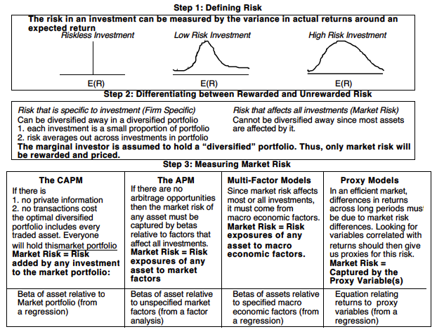
1. Defining Risk
- variance, standard deviation : the spread of the actual returns around the expected return \(var=\frac{Σ(x_i-avg(x))}{n-1}\)
- skewness : the bias towards positive or negative returns
- kurtosis : fatter tails lead to higher kurtosis
- expected return : the opportunity in the investment
- stardard deviation or variance : the danger
→ higher expected returns & more positive skewness is preferred
2. Diversifiable & Non-diversifiable Risk
a) The Componenets of Risk
- firm-specific risk : risk that affects only one or a few firms
- project risk : risk that firm may have misjudged the demand
- competitive risk : arise from competitors providing to be stronger or weaker that anticipated
- sector risk : risks that may affect an entire sector restricted
- market risk : affect many investments ex) interest rate, economy weakens
b) Diversification reduces firm-specific risk?
more diverse assets → smaller percentage to the whole investment
consider two assets a,b:
\[ μ_p=w_aμ_a+(1-w_a)μ_b,\ σ_p^2=w_a^2σ_a^2+(1-w_a)^2σ_b^2+2w_a(1-w_a)σ_aσ_a\rho_{ab},\\ cov_{ab}=σ_1σ_b\rho_{ab}\]
3. Models Measuring Market Risk
A. The Capical Asset Pricing Model (CAPM)
Assumption
- no transactions costs, all assets are traded and investments are infinitely divisible
- everyone has access to the same information and that investors therefore cannot find under or over valued assets in the market place
Measuring the Market Risk of an Individual Asset
- most of the risk in this asset is firm-specific and can be diversified away → this added risk is measured by the covariance of the asset with the market portfolio.
Measuring the Non-Diversifiable Risk
- variance prior to asset i being added : \(σ^2_m\)
- variance after asset i added = \(σ^2_{m'} = w^2_iσ_i^2+(1-w_i)^2σ_m^2+2w_i(1-w_i)cov_{im} \)
- Consequently, the first term in the equation should approach zero, and the second term should approach \(σ^2_m\) , leaving the third term (\( cov_{im}\), the covariance) as the measure of the risk added by individual asset i.
Standardizing Covariances
\[ β_i=\frac{covariance\ of\ asset\ i\ with\ market\ portfolio}{variance\ of\ the\ market\ portfolio} = \frac{cov_{im}}{σ_m^2}\]
Assets that are riskier than average (using this measure of risk) will have betas that are greater than 1 and assets that are less riskier than average will have betas that are less than 1.
Getting Expected Returns
- the expected return of an asset is linearly related to the beta of the asset
\[ E(R_i)=R_f+β_i(E(R_m)-R_f),\ R_f:risk-free\ rate\]
The riskless asset : an asset for which the investor knows the expected return with certainty
The risk premium is the premium demanded by investors for investing in the market portfolio,
The beta, which we defined as the covariance of the asset divided by the variance of the market portfolio, measures the risk added on by an investment to the market portfolio.
B. The Arbitrage Pricing Model
\[ R=E(R)+m+\varepsilon,\ m:market-wide\ risk,\ \varepsilon:firm=specific\ risk\]
The sources of Market-wide Risk
- arbitrage pricing model : allows for multiple sources of market-wide risk and
measures the sensitivity of investments to changes in each source.
\[ R=E(R)+m+\varepsilon =R+(β_j F_j+β_2F_2+...+β_nF_n) + \varepsilon\\ β:sensitivity, \quad f_j:unanticipated change\]
Expected Returns & betas
the beta of a portfolio is the weighted average of the betas of the assets in the portfolio.
This property, in conjunction with the absence of arbitrage, leads to the conclusion that expected returns should be linearly related to betas.
\[ E(R) = R_f+β_i[E(R_i)-R_f]+...+β_n[E(R_n)-R_f]\\ bracket:risk\ premium\]
APM in Practice
- estimated using historical data on asset returns
- It specifies the number of common factors that affected the historical return data
- It measures the beta of each investment relative to each of the common factors and provides an estimate of the actual risk premium earned by each factor.
- the market risk is measured relative to multiple unspecified macroeconomic variables, with the sensitivity of the investment relative to each factor being measured by a beta.
C. Multi-factor Models for risk & return
- Replace the unidentified statistical factors with specific economic factors and the
resultant model should have an economic basis while still retaining much of the strength of the arbitrage pricing model.
ex) \(E(R)=R_f+β_{GNP}[E(R_{GNP})-R_f]+β_I[E(R_I)-R_f]+... \)
- economic factors can change over time, as will the risk premier associated with each one
D. Regression or Proxy Models
- extract their measures of market risk (betas) by looking at historical data
Models of Default Risk
the measurement of default risk and the relationship of default risk to interest rates on borrowing.
the expected return on a corporate bond is likely to reflect the firm-specific default risk of the firm issuing the bond.
Determinants of Default Risk
- the firm’s capacity to generate cash flows from operations
- firms with significant existing investments, which generate relatively high cash flows, will have lower default risk than firms that do not
- its financial obligations
- Firms that operate in predictable and stable businesses will have lower default risk than will other similar firms that operate in cyclical or volatile businesses.
- the firm’s capacity to generate cash flows from operations
Determinants of Bond Ratings → financial ratios
- measure the capacity of the company to meet debt payments and generate stable and predictable cash flows.
\[ pretax\ interest\ coverage = \frac{pretax\ income\ from\ continuing\ operation+interest\ expense}{gross\ interest}\\ EBITDA\ interest\ coverage=\frac{EBITDA}{Gross\ Interest}\\funds\ from\ operation/Total\ debt=\frac{Net\ Income\ from\ Continuing\ operations + Depreciation}{total\ debt}\\ Free\ Operating\ cashflow/total\ debt=\frac{funds\ from\ operations-capital\ expenditures-change\ in\ working\ capital}{total\ debt} \\ Pretax\ Return\ on\ permanent\ capital=\frac{Pretax\ income\ from \ continuing\ operations+interest\ expense}{average\ of \ beg.\ year\ and\ End\ year\ of\ long\ and\ short\ term\ debt,\ minority\ interest\ and \shareholders\ equity} \\ operating\ income/sales=\frac{Sales-COGS-selling\ expenses-administrative\ expenses-R\&D expenses}{sales} \\ long-term\ debt/capital=\frac{long-term\ debt}{long-term\ debt+equity}\\total\ debt/capitalization=\frac{total\ debt}{total\ debt+equity} \]